Example Output

Now that you have completed your alignment based profiling using MiFoDB, we can calculate the mapping abundance.

Table setup

1. Your inStrain profile results

EBC_087.IS_genome_info.csv:

genome	coverage	breadth	nucl_diversity	length	true_scaffolds	detected_scaffolds	coverage_median	coverage_std	coverage_SEM	breadth_minCov	breadth_expected	nucl_diversity_rarefied	conANI_reference	popANI_reference	iRep	iRep_GC_corrected	linked_SNV_count	SNV_distance_mean	r2_mean	d_prime_mean	consensus_divergent_sites	population_divergent_sites	SNS_count	SNV_count	filtered_read_pair_count	reads_unfiltered_pairs	reads_mean_PID	reads_unfiltered_reads	divergent_site_count
C-03.Ssa-BR.fna	1.686020547	0.049164091	0.004595774	1896140	182	86	0	69.19478668	0.050739639	0.011300326	0.774346839	0.000140703	0.986372334	0.988145797		FALSE	242	39.69008264	0.951699521	0.999845137	292	254	252	165	15171	15417	0.981642137	36199	417
EBC_086.5.fna	1.596317454	0.049848898	0.006035971	2377866	79	52	0	19.94120243	0.012974942	0.028909535	0.755746415	0.002048653	0.979081506	0.984682077		FALSE	1337	56.69334331	0.637899652	0.9941014	1438	1053	1040	825	17829	19210	0.969968582	48221	1865

2. Sample read info, found in bowtie2.log file created after making the .bam file. For each bowtie2.log, save the sample name and paired reads (in this example 18233183 before (100.00%) were paired, which is the read_pairs after adapter trimming and human genome remover) .. code-block:

$ head bowtie2.EBC_087.log
  18233183 reads; of these:
    18233183 (100.00%) were paired; of these:
     16282298 (89.30%) aligned concordantly 0 times
     1046019 (5.74%) aligned concordantly exactly 1 time
     904866 (4.96%) aligned concordantly >1 times
     ----
     16282298 pairs aligned concordantly 0 times; of these:
      520393 (3.20%) aligned discordantly 1 time
     ----
     15761905 pairs aligned 0 times concordantly or discordantly; of these:

3. Database mapping file MiFoDB_beta_v2_allRef

Calculate relative abundance:

1. Join the IS_genome_info.csv file to sample read info and sample mapping information.

percent_abundance = ((filtered_read_pair_count)/read_pairs)*100))

Where filtered_read_pair_count is originally in the .IS_genome_info.csv, and read_pairs is from bowtie2.log

It should look something like this:

Example: EBC_087_profile.csv

genome	sample	length	coverage	abundance	breadth	filtered_read_pair_count	read_pairs
EBC_086.5	EBC_087	2377866	2.03925873030692	0.215016678311685	0.150023592582593	38578	17941864
GCF_001039045.1_ASM103904v1_genomic	EBC_087	2899876	1.27013224013716	0.147297961906299	0.019880160393065	26428	17941864
GCF_001434915.1_ASM143491v1_genomic	EBC_087	2232918	0.739709653466898	0.0614707591139917	0.0044753098859877	11029	17941864
GCF_002276885.1_ASM227688v1_genomic	EBC_087	2495148	2.08628466127059	0.218199179304893	0.0112313978970385	39149	17941864
GCF_003641185.1_ASM364118v1_genomic	EBC_087	3671373	1.62835157310358	0.244311293408533	0.0552324702502306	43834	17941864

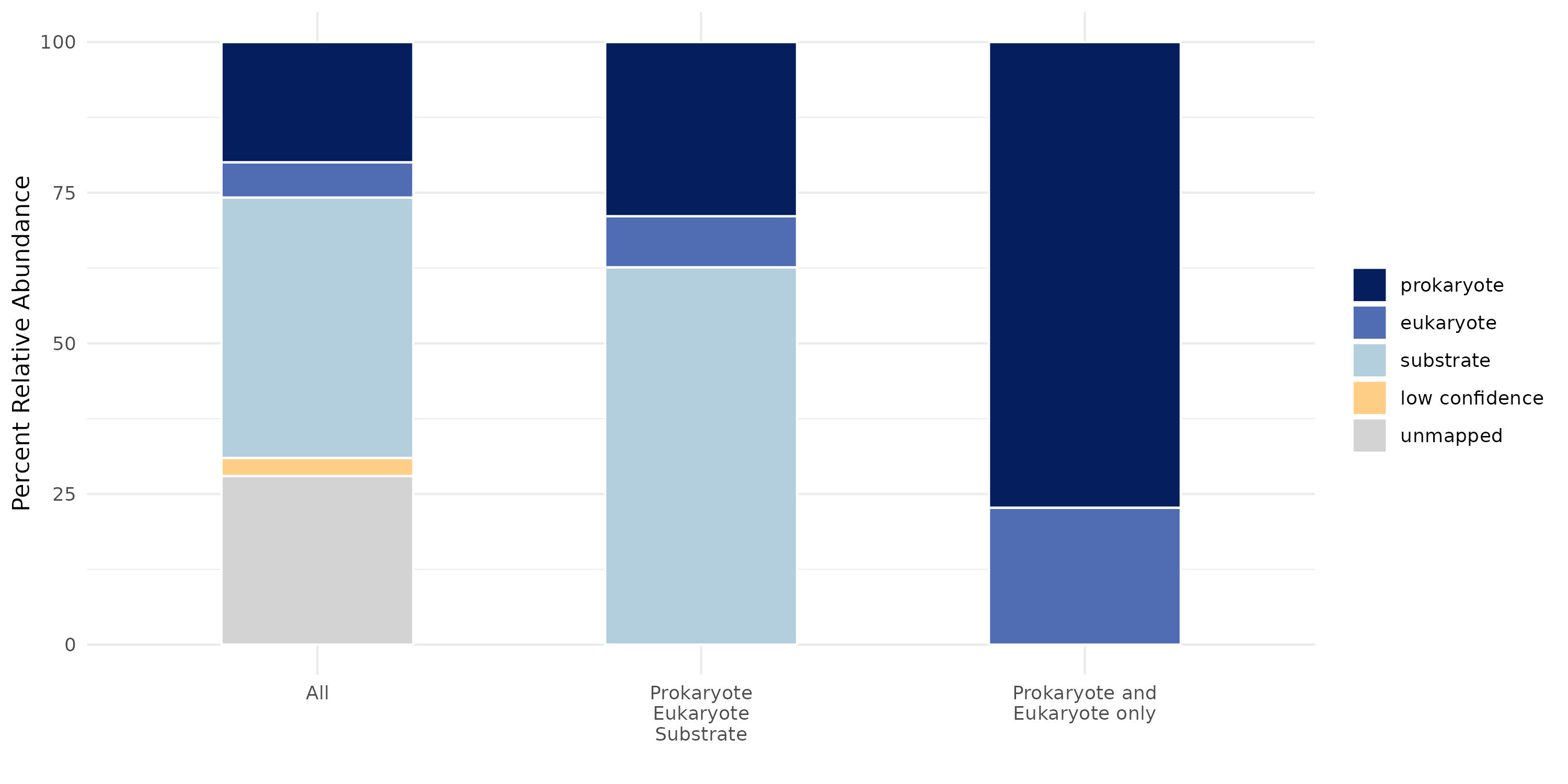
2. For QC, filter any genomes with breadth < 0.5. Those can be considered “low confidence” mapping, while any genomes with breadth > 0.5 are considered high-confidence mapping results.

You can then combine all results from MiFoDB_prok, MiFoDB_euk, and MiFoDB_sub.

For an additional QC with MiFoDB_sub, remove any genome with abundance <2%.

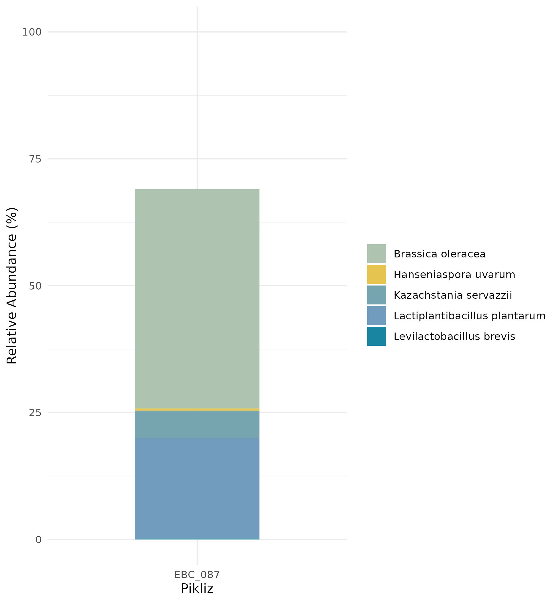
3. Results are now ready for plotting and downstream analysis. For example:

Or take a closer look at the mapped species: